Linear regression (Stan)

We will now conduct the same linear regression as in the previous chapter, but with Stan rather than PyMC. The Stan documentation has an example of linear regression model as well.

import numpy as np
import pandas as pd
import matplotlib.pyplot as plt

import arviz as az
from cmdstanpy import CmdStanModel

Data

df = pd.read_csv('data/linreg.csv')
# Separating pre and post periods
df_train = df[df['period']=="pre"]
df_test = df[df['period']=="post"]

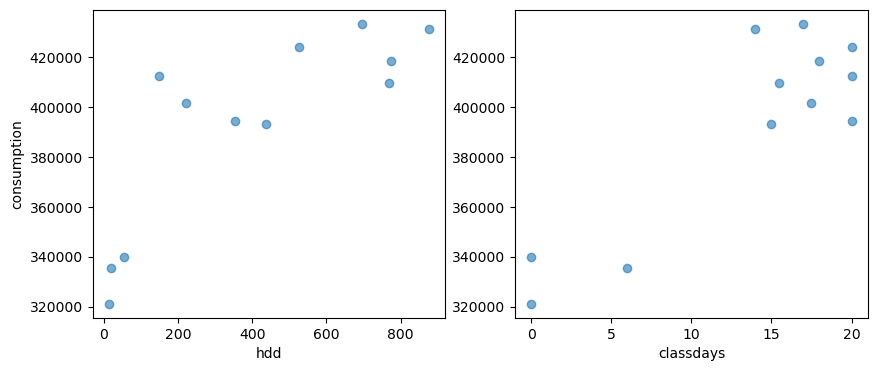
# A plot of the dependent variable vs. each of the explanatory variables
fig, axes = plt.subplots(1, 2, figsize=(10, 4))
axes[0].scatter(df_train['HDD'], df_train['consumption'], alpha=0.6)
axes[1].scatter(df_train['CLASSDAYS'], df_train['consumption'], alpha=0.6)
axes[0].set_ylabel("consumption")
axes[0].set_xlabel("hdd")
axes[1].set_xlabel("classdays")

Text(0.5, 0, 'classdays')

Model specification

A Stan model is a block of text that can either be written in a separate file, or in the same script as the current code. Stan has high-level interfaces with most programming languages. Here, we’ll use CmdStanPy.

data {
  int<lower=0> N;     // number of data items
  int<lower=0> K;     // number of predictors
  matrix[N, K] x;     // predictor matrix
  vector[N] y;        // outcome vector
}
parameters {
  real alpha;           // intercept
  vector[K] beta;       // coefficients for predictors
  real<lower=0> sigma;  // error scale
 }
model {
  y ~ normal(x * beta + alpha, sigma);  // likelihood
}
generated quantities {
  array[N] real log_lik;
  array[N] real y_hat;
  for (j in 1:N) {
    log_lik[j] = normal_lpdf(y[j] | x[j] * beta + alpha, sigma);
    y_hat[j] = normal_rng(x[j] * beta + alpha, sigma);
  }
}

This code should has been written into a dedicated file called linearregression.stan, which we then load:

model = CmdStanModel(stan_file='models/linearregression.stan')

If there is no compiled executable of this model in this filepath, this function will create one. If there is and the model has not been modified, it will load it without recompilation. This allows saving time when fitting the same model: compiling a new or modified model for the first time takes a while, but then the compiled executable is saved and the model may be re-used at will with different data sets.

Training

The sample() method is used to do Bayesian inference over the model conditioned on data using using Hamiltonian Monte Carlo (HMC) sampling. It runs Stan’s HMC-NUTS sampler on the model and data and returns a CmdStanMCMC object. CmdStanPy allows specifying the data as a Python dictionary.

In the PyMC linear regression example, we fit two models: one with only HDD as explanatory variable, and one with also the class days. Let us do the same here:

# Data declaration for model 1
model1_data = {
    "N": len(df_train),
    "K": 1,
    "x": df_train[['HDD']].values,
    "y": df_train['consumption'].values,
}

# Fitting model 1
fit1 = model.sample(data=model1_data, show_progress=False)

09:54:13 - cmdstanpy - INFO - CmdStan start processing
09:54:13 - cmdstanpy - INFO - Chain [1] start processing
09:54:13 - cmdstanpy - INFO - Chain [2] start processing
09:54:13 - cmdstanpy - INFO - Chain [3] start processing
09:54:13 - cmdstanpy - INFO - Chain [4] start processing

09:54:14 - cmdstanpy - INFO - Chain [3] done processing
09:54:15 - cmdstanpy - INFO - Chain [1] done processing
09:54:15 - cmdstanpy - INFO - Chain [4] done processing
09:54:16 - cmdstanpy - INFO - Chain [2] done processing

# Data declaration for model 2
model2_data = {
    "N": len(df_train),
    "K": 2,
    "x": df_train[['HDD', 'CLASSDAYS']].values,
    "y": df_train['consumption'].values,
}

# Fitting model 2
fit2 = model.sample(data=model2_data, show_progress=False)

09:54:16 - cmdstanpy - INFO - CmdStan start processing
09:54:16 - cmdstanpy - INFO - Chain [1] start processing
09:54:16 - cmdstanpy - INFO - Chain [2] start processing
09:54:16 - cmdstanpy - INFO - Chain [3] start processing
09:54:16 - cmdstanpy - INFO - Chain [4] start processing
09:54:18 - cmdstanpy - INFO - Chain [3] done processing
09:54:19 - cmdstanpy - INFO - Chain [4] done processing
09:54:19 - cmdstanpy - INFO - Chain [1] done processing
09:54:19 - cmdstanpy - INFO - Chain [2] done processing

We can see than sampling is quite fast once the model has been compiled.

Note: the show_progress=False argument used above is only to simplify the display on this page. It can be removed or set to True to track the progress of sampling.

CmdStan has diagnostics utilities: stansummary and diagnose

The summary() method runs an utility that reads the outputs of all chains and computes summary statistics for all sampler and model parameters and quantities of interest. It also returns summaries of the total joint log-probability density lp__.

fs = fit1.summary(percentiles=(5, 50, 95))
fs.loc[['alpha', 'beta[1]', 'sigma', 'lp__']]

	Mean	MCSE	StdDev	5%	50%	95%	N_Eff	N_Eff/s	R_hat
alpha	351957.0000	367.627000	13780.000000	329221.000	352384.0000	374190.000	1405.020000	730.259000	0.999853
beta[1]	100.2520	0.697350	26.573900	57.367	99.9952	143.995	1452.140000	754.750000	0.999405
sigma	27345.6132	203.997122	7403.755025	18267.100	25965.8000	41039.000	1317.212973	684.622127	1.000971
lp__	-117.5860	0.044984	1.419820	-120.228	-117.2350	-116.031	996.235000	517.794000	1.002270

fs = fit2.summary(percentiles=(5, 50, 95))
fs.loc[['alpha', 'beta[1]', 'beta[2]', 'sigma', 'lp__']]

	Mean	MCSE	StdDev	5%	50%	95%	N_Eff	N_Eff/s	R_hat
alpha	325605.00000	235.844000	9436.19000	310892.0000	325514.0000	340604.0000	1600.83000	1137.76000	1.004220
beta[1]	56.48890	0.383132	17.16070	29.7856	56.5464	83.7613	2006.19000	1425.86000	0.999786
beta[2]	3261.10000	17.712800	734.32600	2063.7100	3259.4900	4438.6500	1718.71000	1221.55000	1.002670
sigma	14078.61626	125.454950	4278.56431	9125.7000	13254.4000	21583.4000	1163.10931	826.65907	1.003890
lp__	-110.08700	0.062631	1.80114	-113.5180	-109.7060	-108.0380	827.02500	587.79300	1.006430

Additionally, the diagnose() method runs an utility which analyzes the per-draw sampler parameters across all chains looking for potential problems which indicate that the sample isn’t a representative sample from the posterior.

print(fit2.diagnose())

Processing csv files: /tmp/tmplq8zu57i/linearregressionk24hs4cb/linearregression-20250923095416_1.csv, /tmp/tmplq8zu57i/linearregressionk24hs4cb/linearregression-20250923095416_2.csv, /tmp/tmplq8zu57i/linearregressionk24hs4cb/linearregression-20250923095416_3.csv, /tmp/tmplq8zu57i/linearregressionk24hs4cb/linearregression-20250923095416_4.csv

Checking sampler transitions treedepth.
Treedepth satisfactory for all transitions.

Checking sampler transitions for divergences.
No divergent transitions found.

Checking E-BFMI - sampler transitions HMC potential energy.
E-BFMI satisfactory.

Effective sample size satisfactory.

Split R-hat values satisfactory all parameters.

Processing complete, no problems detected.

Extracting results

The fit1 and fit2 objects include methods to access the sampler outputs. They are listed on CmdStanPy’s documentation but we can mention two of them:

• draws_pd(): returns a pandas.DataFrame over all columns in the Stan CSV file. The argument vars can be used to restrict this to one or more variables.

• draws_xr(): returns an xarray.Dataset which maps model variable names to their respective values.

res_pd = fit1.draws_pd()
res_xr = fit1.draws_xr()
res_pd.head()

	chain__	iter__	draw__	lp__	accept_stat__	stepsize__	treedepth__	n_leapfrog__	divergent__	energy__	...	y_hat[3]	y_hat[4]	y_hat[5]	y_hat[6]	y_hat[7]	y_hat[8]	y_hat[9]	y_hat[10]	y_hat[11]	y_hat[12]
0	1.0	1.0	1.0	-118.238	0.971145	0.339103	3.0	7.0	0.0	118.663	...	373191.0	408420.0	449295.0	444354.0	519855.0	458727.0	473612.0	422564.0	345776.0	357898.0
1	1.0	2.0	2.0	-118.237	0.993430	0.339103	4.0	15.0	0.0	119.749	...	355499.0	364834.0	377669.0	427364.0	470069.0	417393.0	413354.0	397723.0	398708.0	354786.0
2	1.0	3.0	3.0	-117.646	0.985189	0.339103	3.0	7.0	0.0	118.872	...	337474.0	403931.0	393499.0	427051.0	424879.0	438156.0	407038.0	403268.0	361106.0	359410.0
3	1.0	4.0	4.0	-118.426	0.659121	0.339103	3.0	7.0	0.0	119.950	...	364002.0	395530.0	387969.0	494433.0	485013.0	462230.0	418238.0	418811.0	447337.0	341333.0
4	1.0	5.0	5.0	-122.657	0.941061	0.339103	3.0	15.0	0.0	123.148	...	479027.0	311505.0	310124.0	368594.0	493771.0	488210.0	505653.0	423499.0	392101.0	304690.0

5 rows × 37 columns

The ArviZ package for exploratory analysis of Bayesian models can be used with CmdStanPy. To make the most out of ArviZ, it is recommended to convert the results to InferenceData. Doing so improves the res_xr xarray by assigning all variables to the right groups.

idata1 = az.from_cmdstanpy(
    posterior = fit1,
    posterior_predictive="y_hat",
    observed_data={"y": df_train['consumption'].values},
    constant_data={"x": df_train[['HDD']].values},
    log_likelihood="log_lik",
    dims={
        "y_hat": ["observations"],
        "log_lik": ["observations"],
        "y": ["observations"],
        "beta": ["features"]
        },
)

idata2 = az.from_cmdstanpy(
    posterior = fit2,
    posterior_predictive="y_hat",
    observed_data={"y": df_train['consumption'].values},
    constant_data={"x": df_train[['HDD', 'CLASSDAYS']].values},
    log_likelihood="log_lik",
    dims={
        "y_hat": ["observations"],
        "log_lik": ["observations"],
        "y": ["observations"],
        "beta": ["features"]
        },
)

idata2

arviz.InferenceData

• posterior

  <xarray.Dataset> Size: 136kB
  Dimensions:   (chain: 4, draw: 1000, features: 2)
  Coordinates:
    * chain     (chain) int64 32B 0 1 2 3
    * draw      (draw) int64 8kB 0 1 2 3 4 5 6 7 ... 993 994 995 996 997 998 999
    * features  (features) int64 16B 0 1
  Data variables:
      alpha     (chain, draw) float64 32kB 3.308e+05 3.232e+05 ... 3.237e+05
      beta      (chain, draw, features) float64 64kB 26.95 3.918e+03 ... 3.976e+03
      sigma     (chain, draw) float64 32kB 1.053e+04 1.226e+04 ... 1.716e+04
  Attributes:
      created_at:                 2025-09-23T07:54:26.529345+00:00
      arviz_version:              0.22.0
      inference_library:          cmdstanpy
      inference_library_version:  1.2.5

  xarray.Dataset

  • Dimensions:
    • chain: 4
    • draw: 1000
    • features: 2
  • Coordinates: (3)
    • chain
      (chain)
      int64
      0 1 2 3

      array([0, 1, 2, 3])

    • draw
      (draw)
      int64
      0 1 2 3 4 5 ... 995 996 997 998 999

      array([  0,   1,   2, ..., 997, 998, 999])

    • features
      (features)
      int64
      0 1

      array([0, 1])

  • Data variables: (3)
    • alpha
      (chain, draw)
      float64
      3.308e+05 3.232e+05 ... 3.237e+05

      array([[330838., 323206., 319306., ..., 345713., 331582., 331593.],
             [331632., 333973., 338949., ..., 327456., 325632., 329063.],
             [318270., 317650., 329469., ..., 326005., 319475., 326079.],
             [322317., 321656., 325487., ..., 325204., 319794., 323720.]])

    • beta
      (chain, draw, features)
      float64
      26.95 3.918e+03 ... 43.96 3.976e+03

      array([[[  26.9524, 3917.51  ],
              [  41.6824, 3917.27  ],
              [  60.4771, 3280.63  ],
              ...,
              [  82.767 , 1601.05  ],
              [  75.7133, 2530.87  ],
              [  69.0617, 2310.88  ]],
      
             [[  50.0078, 3082.69  ],
              [  45.1202, 3098.94  ],
              [  36.0891, 3386.    ],
              ...,
              [  59.5503, 3415.7   ],
              [  46.1124, 3852.4   ],
              [  68.2127, 2928.8   ]],
      
             [[  71.738 , 2523.8   ],
              [  85.9264, 2885.56  ],
              [  52.9445, 2705.44  ],
              ...,
              [  35.6302, 3359.29  ],
              [  70.0646, 2863.45  ],
              [  46.1583, 3634.09  ]],
      
             [[  42.8418, 3612.11  ],
              [  41.2594, 4031.52  ],
              [  74.3224, 2986.    ],
              ...,
              [  66.2989, 2987.39  ],
              [  69.4294, 3334.72  ],
              [  43.9627, 3976.28  ]]])

    • sigma
      (chain, draw)
      float64
      1.053e+04 1.226e+04 ... 1.716e+04

      array([[10532.2 , 12255.2 , 11354.2 , ..., 18724.7 , 12636.5 , 15210.4 ],
             [14360.5 , 14450.5 , 14354.4 , ...,  9340.34, 12777.4 , 10174.8 ],
             [25981.  , 28797.6 , 18295.3 , ..., 18223.2 , 10000.9 ,  9285.44],
             [11201.  , 10314.8 , 15617.8 , ..., 16538.6 , 10392.4 , 17164.3 ]])

  • Indexes: (3)
    • chain
      PandasIndex

      PandasIndex(Index([0, 1, 2, 3], dtype='int64', name='chain'))

    • draw
      PandasIndex

      PandasIndex(Index([  0,   1,   2,   3,   4,   5,   6,   7,   8,   9,
             ...
             990, 991, 992, 993, 994, 995, 996, 997, 998, 999],
            dtype='int64', name='draw', length=1000))

    • features
      PandasIndex

      PandasIndex(Index([0, 1], dtype='int64', name='features'))

  • Attributes: (4)

    created_at :

    2025-09-23T07:54:26.529345+00:00

    arviz_version :

    0.22.0

    inference_library :

    cmdstanpy

    inference_library_version :

    1.2.5

  
  
• posterior_predictive

  <xarray.Dataset> Size: 392kB
  Dimensions:       (chain: 4, draw: 1000, observations: 12)
  Coordinates:
    * chain         (chain) int64 32B 0 1 2 3
    * draw          (draw) int64 8kB 0 1 2 3 4 5 6 ... 993 994 995 996 997 998 999
    * observations  (observations) int64 96B 0 1 2 3 4 5 6 7 8 9 10 11
  Data variables:
      y_hat         (chain, draw, observations) float64 384kB 3.307e+05 ... 3.3...
  Attributes:
      created_at:                 2025-09-23T07:54:26.630012+00:00
      arviz_version:              0.22.0
      inference_library:          cmdstanpy
      inference_library_version:  1.2.5

  xarray.Dataset

  • Dimensions:
    • chain: 4
    • draw: 1000
    • observations: 12
  • Coordinates: (3)
    • chain
      (chain)
      int64
      0 1 2 3

      array([0, 1, 2, 3])

    • draw
      (draw)
      int64
      0 1 2 3 4 5 ... 995 996 997 998 999

      array([  0,   1,   2, ..., 997, 998, 999])

    • observations
      (observations)
      int64
      0 1 2 3 4 5 6 7 8 9 10 11

      array([ 0,  1,  2,  3,  4,  5,  6,  7,  8,  9, 10, 11])

  • Data variables: (1)
    • y_hat
      (chain, draw, observations)
      float64
      3.307e+05 3.435e+05 ... 3.302e+05

      array([[[330681., 343525., 393982., ..., 414709., 398006., 343061.],
              [316430., 344956., 402098., ..., 384249., 396386., 344307.],
              [296884., 363780., 401278., ..., 384572., 384467., 335004.],
              ...,
              [348065., 366779., 381558., ..., 357352., 378472., 350140.],
              [339767., 326483., 396365., ..., 404434., 392213., 341052.],
              [327178., 328944., 389899., ..., 407677., 408970., 322385.]],
      
             [[336532., 344901., 424486., ..., 390738., 387103., 356405.],
              [357973., 345658., 421779., ..., 388161., 392031., 356084.],
              [321621., 361362., 398378., ..., 392875., 403697., 348529.],
              ...,
              [317600., 338556., 411321., ..., 409916., 395733., 343547.],
              [306752., 362489., 406663., ..., 397131., 407932., 333656.],
              [353331., 373565., 391730., ..., 413654., 399564., 307822.]],
      
             [[274092., 312471., 333920., ..., 383993., 361140., 308700.],
              [296098., 342804., 350877., ..., 416851., 334984., 289208.],
              [334866., 336931., 399435., ..., 378343., 358856., 341014.],
              ...,
              [334789., 329058., 406859., ..., 388288., 396275., 356341.],
              [329520., 343501., 387524., ..., 389012., 388353., 320014.],
              [326219., 342364., 405749., ..., 397236., 411667., 327611.]],
      
             [[298516., 344848., 388602., ..., 386560., 400838., 317840.],
              [327759., 341034., 422881., ..., 406887., 415242., 305080.],
              [327232., 342776., 385321., ..., 390542., 378867., 357817.],
              ...,
              [327481., 337429., 397955., ..., 408940., 423798., 325057.],
              [321359., 336362., 384823., ..., 396656., 394181., 325175.],
              [314879., 349848., 412669., ..., 386912., 391147., 330234.]]])

  • Indexes: (3)
    • chain
      PandasIndex

      PandasIndex(Index([0, 1, 2, 3], dtype='int64', name='chain'))

    • draw
      PandasIndex

      PandasIndex(Index([  0,   1,   2,   3,   4,   5,   6,   7,   8,   9,
             ...
             990, 991, 992, 993, 994, 995, 996, 997, 998, 999],
            dtype='int64', name='draw', length=1000))

    • observations
      PandasIndex

      PandasIndex(Index([0, 1, 2, 3, 4, 5, 6, 7, 8, 9, 10, 11], dtype='int64', name='observations'))

  • Attributes: (4)

    created_at :

    2025-09-23T07:54:26.630012+00:00

    arviz_version :

    0.22.0

    inference_library :

    cmdstanpy

    inference_library_version :

    1.2.5

  
  
• log_likelihood

  <xarray.Dataset> Size: 392kB
  Dimensions:       (chain: 4, draw: 1000, observations: 12)
  Coordinates:
    * chain         (chain) int64 32B 0 1 2 3
    * draw          (draw) int64 8kB 0 1 2 3 4 5 6 ... 993 994 995 996 997 998 999
    * observations  (observations) int64 96B 0 1 2 3 4 5 6 7 8 9 10 11
  Data variables:
      log_lik       (chain, draw, observations) float64 384kB -10.64 ... -10.99
  Attributes:
      created_at:                 2025-09-23T07:54:26.666022+00:00
      arviz_version:              0.22.0
      inference_library:          cmdstanpy
      inference_library_version:  1.2.5

  xarray.Dataset

  • Dimensions:
    • chain: 4
    • draw: 1000
    • observations: 12
  • Coordinates: (3)
    • chain
      (chain)
      int64
      0 1 2 3

      array([0, 1, 2, 3])

    • draw
      (draw)
      int64
      0 1 2 3 4 5 ... 995 996 997 998 999

      array([  0,   1,   2, ..., 997, 998, 999])

    • observations
      (observations)
      int64
      0 1 2 3 4 5 6 7 8 9 10 11

      array([ 0,  1,  2,  3,  4,  5,  6,  7,  8,  9, 10, 11])

  • Data variables: (1)
    • log_lik
      (chain, draw, observations)
      float64
      -10.64 -11.87 ... -10.67 -10.99

      array([[[-10.6373, -11.8681, -10.1828, ..., -10.4872, -10.2392,
               -10.4375],
              [-10.3554, -10.8119, -10.4112, ..., -10.4972, -10.3347,
               -11.0206],
              [-10.2605, -10.3399, -11.6147, ..., -10.2686, -10.7857,
               -11.4111],
              ...,
              [-11.6943, -11.4099, -11.4856, ..., -10.9873, -10.892 ,
               -10.9096],
              [-10.7719, -10.8696, -11.5159, ..., -10.6434, -10.6262,
               -10.4173],
              [-10.8271, -10.8236, -11.8519, ..., -10.5717, -11.0013,
               -10.5925]],
      
             [[-10.7924, -11.0795, -10.8341, ..., -10.5958, -10.5551,
               -10.5645],
              [-10.929 , -11.2665, -10.7344, ..., -10.6155, -10.5283,
               -10.5255],
              [-11.3022, -11.9408, -10.4915, ..., -10.8617, -10.5381,
               -10.4935],
      ...
              [-10.7723, -10.9228, -11.0291, ..., -10.7315, -10.854 ,
               -10.9427],
              [-10.1322, -10.1605, -13.3734, ..., -10.1294, -11.523 ,
               -11.5015],
              [-10.2335, -11.0747, -10.3382, ..., -10.3909, -10.0758,
               -10.7903]],
      
             [[-10.2548, -10.5874, -10.7861, ..., -10.2598, -10.4252,
               -11.1636],
              [-10.1656, -10.742 , -10.2425, ..., -10.3913, -10.1612,
               -11.3554],
              [-10.6329, -10.7533, -11.1253, ..., -10.7634, -10.6935,
               -10.7936],
              ...,
              [-10.6768, -10.777 , -11.213 , ..., -10.6943, -10.8019,
               -10.8553],
              [-10.1687, -10.3145, -11.327 , ..., -10.3938, -10.4845,
               -11.3952],
              [-10.6865, -10.9524, -10.6831, ..., -10.8203, -10.6722,
               -10.9898]]])

  • Indexes: (3)
    • chain
      PandasIndex

      PandasIndex(Index([0, 1, 2, 3], dtype='int64', name='chain'))

    • draw
      PandasIndex

      PandasIndex(Index([  0,   1,   2,   3,   4,   5,   6,   7,   8,   9,
             ...
             990, 991, 992, 993, 994, 995, 996, 997, 998, 999],
            dtype='int64', name='draw', length=1000))

    • observations
      PandasIndex

      PandasIndex(Index([0, 1, 2, 3, 4, 5, 6, 7, 8, 9, 10, 11], dtype='int64', name='observations'))

  • Attributes: (4)

    created_at :

    2025-09-23T07:54:26.666022+00:00

    arviz_version :

    0.22.0

    inference_library :

    cmdstanpy

    inference_library_version :

    1.2.5

  
  
• sample_stats

  <xarray.Dataset> Size: 204kB
  Dimensions:          (chain: 4, draw: 1000)
  Coordinates:
    * chain            (chain) int64 32B 0 1 2 3
    * draw             (draw) int64 8kB 0 1 2 3 4 5 6 ... 994 995 996 997 998 999
  Data variables:
      lp               (chain, draw) float64 32kB -110.9 -108.5 ... -108.6 -109.9
      acceptance_rate  (chain, draw) float64 32kB 1.0 0.9958 ... 0.9849 0.9353
      step_size        (chain, draw) float64 32kB 0.1959 0.1959 ... 0.2104 0.2104
      tree_depth       (chain, draw) int64 32kB 2 3 3 4 4 3 3 4 ... 4 4 5 3 3 4 4
      n_steps          (chain, draw) int64 32kB 3 7 11 31 15 11 ... 31 15 15 15 15
      diverging        (chain, draw) bool 4kB False False False ... False False
      energy           (chain, draw) float64 32kB 116.9 111.3 ... 109.9 112.2
  Attributes:
      created_at:                 2025-09-23T07:54:26.586935+00:00
      arviz_version:              0.22.0
      inference_library:          cmdstanpy
      inference_library_version:  1.2.5

  xarray.Dataset

  • Dimensions:
    • chain: 4
    • draw: 1000
  • Coordinates: (2)
    • chain
      (chain)
      int64
      0 1 2 3

      array([0, 1, 2, 3])

    • draw
      (draw)
      int64
      0 1 2 3 4 5 ... 995 996 997 998 999

      array([  0,   1,   2, ..., 997, 998, 999])

  • Data variables: (7)
    • lp
      (chain, draw)
      float64
      -110.9 -108.5 ... -108.6 -109.9

      array([[-110.895, -108.522, -108.643, ..., -112.852, -109.45 , -109.591],
             [-108.669, -109.016, -110.682, ..., -109.888, -108.889, -108.948],
             [-114.066, -114.159, -110.744, ..., -111.336, -110.588, -108.523],
             [-109.023, -108.906, -109.624, ..., -109.311, -108.614, -109.932]])

    • acceptance_rate
      (chain, draw)
      float64
      1.0 0.9958 0.8233 ... 0.9849 0.9353

      array([[1.      , 0.995838, 0.823321, ..., 0.871905, 0.987154, 0.995398],
             [0.997264, 0.999074, 0.874366, ..., 0.992823, 0.793126, 0.966091],
             [0.889025, 0.814098, 0.983073, ..., 0.932783, 0.977541, 0.864713],
             [0.995465, 0.696758, 0.798966, ..., 0.990618, 0.984888, 0.935284]])

    • step_size
      (chain, draw)
      float64
      0.1959 0.1959 ... 0.2104 0.2104

      array([[0.195888, 0.195888, 0.195888, ..., 0.195888, 0.195888, 0.195888],
             [0.212446, 0.212446, 0.212446, ..., 0.212446, 0.212446, 0.212446],
             [0.242326, 0.242326, 0.242326, ..., 0.242326, 0.242326, 0.242326],
             [0.210444, 0.210444, 0.210444, ..., 0.210444, 0.210444, 0.210444]])

    • tree_depth
      (chain, draw)
      int64
      2 3 3 4 4 3 3 4 ... 4 4 4 5 3 3 4 4

      array([[2, 3, 3, ..., 4, 4, 4],
             [2, 3, 3, ..., 4, 4, 3],
             [3, 3, 4, ..., 4, 4, 3],
             [4, 2, 4, ..., 3, 4, 4]])

    • n_steps
      (chain, draw)
      int64
      3 7 11 31 15 11 ... 31 15 15 15 15

      array([[ 3,  7, 11, ..., 31, 15, 15],
             [ 7,  7,  7, ..., 15, 15, 11],
             [15, 15, 15, ..., 15, 15, 15],
             [15,  3, 15, ..., 15, 15, 15]])

    • diverging
      (chain, draw)
      bool
      False False False ... False False

      array([[False, False, False, ..., False, False, False],
             [False, False, False, ..., False, False, False],
             [False, False, False, ..., False, False, False],
             [False, False, False, ..., False, False, False]])

    • energy
      (chain, draw)
      float64
      116.9 111.3 110.8 ... 109.9 112.2

      array([[116.907, 111.328, 110.751, ..., 114.767, 113.365, 110.425],
             [111.819, 109.103, 111.669, ..., 114.818, 112.226, 111.11 ],
             [117.482, 115.341, 115.873, ..., 112.944, 112.423, 112.848],
             [110.051, 113.752, 111.143, ..., 114.358, 109.942, 112.169]])

  • Indexes: (2)
    • chain
      PandasIndex

      PandasIndex(Index([0, 1, 2, 3], dtype='int64', name='chain'))

    • draw
      PandasIndex

      PandasIndex(Index([  0,   1,   2,   3,   4,   5,   6,   7,   8,   9,
             ...
             990, 991, 992, 993, 994, 995, 996, 997, 998, 999],
            dtype='int64', name='draw', length=1000))

  • Attributes: (4)

    created_at :

    2025-09-23T07:54:26.586935+00:00

    arviz_version :

    0.22.0

    inference_library :

    cmdstanpy

    inference_library_version :

    1.2.5

  
  
• observed_data

  <xarray.Dataset> Size: 192B
  Dimensions:       (observations: 12)
  Coordinates:
    * observations  (observations) int64 96B 0 1 2 3 4 5 6 7 8 9 10 11
  Data variables:
      y             (observations) int64 96B 321120 335520 ... 401760 339840
  Attributes:
      created_at:                 2025-09-23T07:54:26.640046+00:00
      arviz_version:              0.22.0
      inference_library:          cmdstanpy
      inference_library_version:  1.2.5

  xarray.Dataset

  • Dimensions:
    • observations: 12
  • Coordinates: (1)
    • observations
      (observations)
      int64
      0 1 2 3 4 5 6 7 8 9 10 11

      array([ 0,  1,  2,  3,  4,  5,  6,  7,  8,  9, 10, 11])

  • Data variables: (1)
    • y
      (observations)
      int64
      321120 335520 ... 401760 339840

      array([321120, 335520, 412560, 394560, 424080, 409680, 431280, 418320,
             433440, 393120, 401760, 339840])

  • Indexes: (1)
    • observations
      PandasIndex

      PandasIndex(Index([0, 1, 2, 3, 4, 5, 6, 7, 8, 9, 10, 11], dtype='int64', name='observations'))

  • Attributes: (4)

    created_at :

    2025-09-23T07:54:26.640046+00:00

    arviz_version :

    0.22.0

    inference_library :

    cmdstanpy

    inference_library_version :

    1.2.5

  
  
• constant_data

  <xarray.Dataset> Size: 304B
  Dimensions:  (x_dim_0: 12, x_dim_1: 2)
  Coordinates:
    * x_dim_0  (x_dim_0) int64 96B 0 1 2 3 4 5 6 7 8 9 10 11
    * x_dim_1  (x_dim_1) int64 16B 0 1
  Data variables:
      x        (x_dim_0, x_dim_1) float64 192B 12.7 0.0 19.4 6.0 ... 17.5 54.2 0.0
  Attributes:
      created_at:                 2025-09-23T07:54:26.652370+00:00
      arviz_version:              0.22.0
      inference_library:          cmdstanpy
      inference_library_version:  1.2.5

  xarray.Dataset

  • Dimensions:
    • x_dim_0: 12
    • x_dim_1: 2
  • Coordinates: (2)
    • x_dim_0
      (x_dim_0)
      int64
      0 1 2 3 4 5 6 7 8 9 10 11

      array([ 0,  1,  2,  3,  4,  5,  6,  7,  8,  9, 10, 11])

    • x_dim_1
      (x_dim_1)
      int64
      0 1

      array([0, 1])

  • Data variables: (1)
    • x
      (x_dim_0, x_dim_1)
      float64
      12.7 0.0 19.4 6.0 ... 17.5 54.2 0.0

      array([[ 12.7,   0. ],
             [ 19.4,   6. ],
             [147.6,  20. ],
             [353.4,  20. ],
             [526.7,  20. ],
             [767.5,  15.5],
             [876. ,  14. ],
             [773.7,  18. ],
             [696.8,  17. ],
             [436.3,  15. ],
             [220.9,  17.5],
             [ 54.2,   0. ]])

  • Indexes: (2)
    • x_dim_0
      PandasIndex

      PandasIndex(Index([0, 1, 2, 3, 4, 5, 6, 7, 8, 9, 10, 11], dtype='int64', name='x_dim_0'))

    • x_dim_1
      PandasIndex

      PandasIndex(Index([0, 1], dtype='int64', name='x_dim_1'))

  • Attributes: (4)

    created_at :

    2025-09-23T07:54:26.652370+00:00

    arviz_version :

    0.22.0

    inference_library :

    cmdstanpy

    inference_library_version :

    1.2.5

  
  

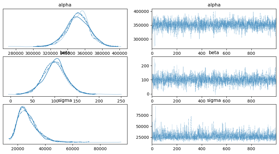
We can now use the same posterior plots as we did with the PyMC output:

az.plot_trace(idata1)

array([[<Axes: title={'center': 'alpha'}>,
        <Axes: title={'center': 'alpha'}>],
       [<Axes: title={'center': 'beta'}>,
        <Axes: title={'center': 'beta'}>],
       [<Axes: title={'center': 'sigma'}>,
        <Axes: title={'center': 'sigma'}>]], dtype=object)

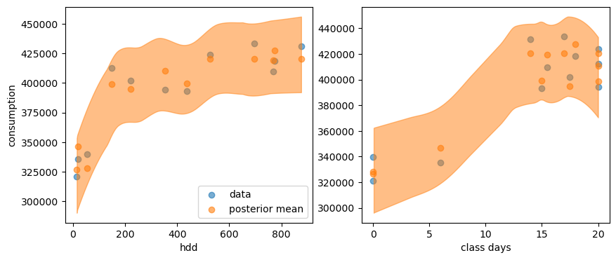
And here is the posterior predictive distribution:

y_post = idata2.posterior_predictive["y_hat"]

fig, axes = plt.subplots(1, 2, figsize=(10, 4))

axes[0].scatter(df_train['HDD'], df_train['consumption'], alpha=0.6, label='data')
axes[0].scatter(df_train['HDD'], y_post.mean(("chain", "draw")), c="C1", alpha=0.6, label='posterior mean')
az.plot_hdi(df_train['HDD'], y_post, ax=axes[0])
axes[0].set_xlabel("hdd")
axes[0].set_ylabel("consumption")
axes[0].legend()

axes[1].scatter(df_train['CLASSDAYS'], df_train['consumption'], alpha=0.6)
axes[1].scatter(df_train['CLASSDAYS'], y_post.mean(("chain", "draw")), c="C1", alpha=0.6)
az.plot_hdi(df_train['CLASSDAYS'], y_post, ax=axes[1])
axes[1].set_xlabel("class days")

Text(0.5, 0, 'class days')

Reassuringly, this looks exactly like the posterior distribution we had from PyMC.

Model comparison metrics

The built-in LOO method of ArviZ can be used now (see the previous chapter for a reminder of what is happening here):

df_comp_loo = az.compare({"model1": idata1, "model2": idata2}, ic="loo")
df_comp_loo

/home/simon/anaconda3/envs/bayes_env/lib/python3.11/site-packages/arviz/stats/stats.py:797: UserWarning: Estimated shape parameter of Pareto distribution is greater than 0.70 for one or more samples. You should consider using a more robust model, this is because importance sampling is less likely to work well if the marginal posterior and LOO posterior are very different. This is more likely to happen with a non-robust model and highly influential observations.
  warnings.warn(

	rank	elpd_loo	p_loo	elpd_diff	weight	se	dse	warning	scale
model2	0	-132.533091	3.046308	0.000000	1.0	1.155242	0.000000	True	log
model1	1	-140.311554	2.490824	7.778464	0.0	2.074431	2.016874	False	log