Time series models

Motivation

Ordinary linear regression (OLR) is based on an assumption of temporal independence: each observation of energy use \(y_t\) is only explained by current explanatory variables \(x_t\) (weather, occupancy). Consecutive values \(y_t,y_{t-1}, y_{t-2}, \dots\) are independent given these input conditions.

After model training, this hypothesis is validated by checking residuals between model output \(\hat{y}_t\) and measurements \(y_t\):

(27)\[\varepsilon_t= \hat{y}_t-y_t\]

The series of residuals \((\varepsilon_1 ,\varepsilon_2 ,\dots,\varepsilon_t)\) should exhibit low values of autocorrelation, to confirm that the remaining model error after training has white noise properties. The autocorrelation function (ACF) of residuals showing significant values hints that the model did not fully capture the data-generating process. In such cases, OLR estimates of savings uncertainty will be biased and underestimated unless corrected.

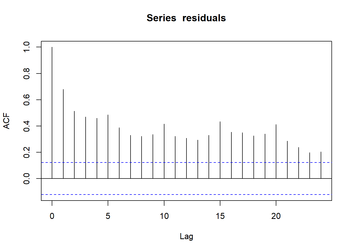
The tutorial on change-point models ended with an ACF graph looking like this:

Fig. 19 ACF exhibiting some high values

In this example, the ACF value is near 0.7 at lag 1: on average, consecutive residuals have a correlation coefficient of 0.7. The lag 2 ACF shows that correlation remains, two observations apart, with an average coefficient over 0.5. The lag 0 ACF is always exactly 1, since each residual is perfectly correlated with itself.

Autocorrelation occurs with high or medium frequency data. For instance, using daily meter readings, a simple linear regression model may overlook the thermal inertia of the building, which makes the daily consumption dependent on the conditions of the previous day to some extent. With higher frequency data (hourly or subhourly), OLR may not longer be applicable at all.

Time series models

Time-series models address high frequency data by formulating relationships between consecutive measurements, up to a certain order.

Autoregressive models: AR, ARX

An Autoregressive model of order \(p\), denoted AR(p), states that the current energy use \(y_t\) depends on its past values, up to a certain lag \(p\):

(28)\[y_t = \varphi_1 y_{t-1} + \varphi_2 y_{t-2} + \dots + \varphi_p y_{t-p} + \varepsilon_t\]

with \(\varepsilon_t \sim N(0, \sigma)\). The \(\varphi\) coefficients are model parameters, to be learned by fitting the model.

This model easily extends into the ARX formulation: autoregressive with exogenous variables.

(29)\[y_t = \sum_{i=1}^p \varphi_i y_{t-i} + \sum_{k=0}^r \beta_k x_{t-k} + \varepsilon_t\]

Where \(x_{t-k}\) are the external factors like weather, occupancy, other heat sources etc. at time \(t - k\). The maximum order \(r\) to which previous values of exogenous variables are included in the equation may be equal to \(p\), or different.

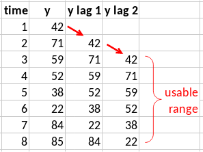
Training an AR or ARX model is straightforward: one simply has to generate a lagged copy of the series \(\{y_t\}\), and include this copy in the explanatory variables of an OLR model.

In this example, lagged copies of \(y\) are created up to an order \(p=2\). The new series are model inputs of a linear regression model. Other variables \(x\) may be added, even with lagged copies. However, the first two data points are no longer usable for training as they are missing some explanatory variables.

This extension of the OLR model is sometimes called the Cochrane-Orcutt procedure. It does not guarantee solving autocorrelation issues: the ACF should still be checked after training.

Moving average models: MA, ARMA, ARMAX

A Moving Average model of order \(q\), MA(q), states that each term of the series \(y_t\) depends on previous values of the error \(\varepsilon_t= \hat{y}_t-y_t\):

(30)\[y_t = \sum_{j=1}^q \theta_j \varepsilon_{t-j} + \varepsilon_t\]

The combination of autoregressive and moving average terms yields the ARMA(p,q) model:

(31)\[y_t = \sum_{i=1}^p \varphi_i y_{t-i} + \sum_{j=1}^q \theta_j \varepsilon_{t-j} + \varepsilon_t\]

Or the ARMAX(p,q) model, if exogenous variables are to be included as well:

(32)\[y_t = \sum_{i=1}^p \varphi_i y_{t-i} + \sum_{j=1}^q \theta_j \varepsilon_{t-j} + \sum_{k=0}^r \beta_k x_{t-k} + \varepsilon_t\]

Unlike an ARX model, any time-series model including a MA component may not be trained as simply as an OLR model, because residuals must be calculated iteratively. Implementations of these models are available in most programming languages.

In a given situation, the choice between an ARX or ARMAX model is not trivial. In practice, one should start with the lowest order, and train models of increasing orders p and q until the ACF criterion is satisfied. In case high autocorrelations have been identified at higher lag values (for instance, with daily data, a lag-7 autocorrelation suggests a weekly pattern not captured by the model), these orders may be included even if lower orders are not.

Prediction uncertainty

Let us suppose that a time series model is trained on a finite dataset \(\{y_t, t\in 1 \dots T\}\), and we now wish to forecast values \(\hat{y}_{T+h}\) up to a certain prediction horizon \(h\). This is referred to as multi-step ahead prediction. This is required for instance in a M&V workflow, to predict energy use during the reporting period.

The models presented here predict \(\hat{y}_t\) from previous measurements \(y_{t-i}\) which are no longer available. A multi-step ahead forecast is:

(33)\[p(y_{T+h} | y_{1:T}) = N(\hat{y}_{T+h}, \sigma_h)\]

where the training dataset stops at the time index \(T\), and \(h\) is the number of steps into the test dataset where the mean \(\hat{y}_{t+h}\) and uncertainty \(\sigma_h\) of the prediction are calculated.

The prediction mean \(\hat{y}_{T+h}\) is obtained from Eq. (32) (or any of the previous models). As the prediction horizon \(h\) increases and measurements are no longer available, the observed terms \(y_{T+h-i}\) are gradually replaced by previous forecast means \(\hat{y}\), and the error terms \(\varepsilon_{T+h-i}\) are set to zero.

However, in order to account for the forecasting uncertainty, increasing with the horizon \(h\), multiple step ahead predictions of ARMA models have an increased variance:

(34)\[\sigma_h^2 = \sigma^2 \sum_{i=0}^{h-1} \psi_i^2\]

where \(\psi_i\) are the coefficients of the MA(\(\infty\)) representation of the ARMA(p,q) process [Shumway et al., 2000]. Eq. (31) can be formulated as a MA(\(\infty\)) process, with coefficients \(\psi\) as functions of the ARMA coefficients \(\varphi\) and \(\theta\):

(35)\[y_t = \varepsilon_t + \sum_{i=1}^\infty \psi_i \varepsilon_{t-i} \]

(36)\[\psi_i = \sum_{j=1}^p \varphi_j \psi_{i-j} +\theta_i\]

and \(\psi_0=1\).

In the generic case, the \(\psi\) coefficients are calculated iteratively, as one new value is required for each new forecast. In the particular case of MA(q) models, the forecast uncertainty is simple to formulate because each \(\psi_i\) is equal to a \(\theta_i\) coefficient. In the particular case of the ARMA(1,1) model, there is a specific formulation of \(\sigma_h\):

(37)\[\sigma_h^2 = \sigma^2 \left[1 + \frac{\left(\varphi+\theta\right)\left(1-\varphi^{2(h-1)}\right)}{1-\varphi^2}\right]\]