A Bayesian data analysis workflow

Motivation for a Bayesian approach

Bayesian statistics are mentioned in the Annex B of the ASHRAE Guideline 14, after it has been observed that standard approaches make it difficult to estimate the savings uncertainty when complex models are required in a measurement and verification worflow:

“Savings uncertainty can only be determined exactly when energy use is a linear function of some independent variable(s). For more complicated models of energy use, such as changepoint models, and for data with serially autocorrelated errors, approximate formulas must be used. These approximations provide reasonable accuracy when compared with simulated data, but in general it is difficult to determine their accuracy in any given situation. One alternative method for determining savings uncertainty to any desired degree of accuracy is to use a Bayesian approach.”

Still on the topic of measurement and verification, and the estimation of savings uncertainty, several advantages and drawbacks of Bayesian approaches are described by [Carstens et al., 2018]. Advantages include:

• Because Bayesian models are probabilistic, uncertainty is automatically and exactly quantified. Confidence intervals can be interpreted in the way most people understand them: degrees of belief about the value of the parameter.

• Bayesian models are more universal and flexible than standard methods. Models are also modular and can be designed to suit the problem. For example, it is no different to create terms for serial correlation, or heteroscedasticity (non-constant variance) than it is to specify an ordinary linear model.

• The Bayesian approach allows for the incorporation of prior information where appropriate.

• When the savings need to be calculated for “normalised conditions”, for example, a “typical meteorological year”, rather than the conditions during the post-retrofit monitoring period, it is not possible to quantify uncertainty using current methods. However, it can be naturally and easily quantified using the Bayesian approach.

The first two points above are the most relevant to a data analyst: any arbitrary model structure can be defined to explain the data, and the exact same set of formulas can then be used to obtain any uncertainty after the models have been fitted.

Workflow

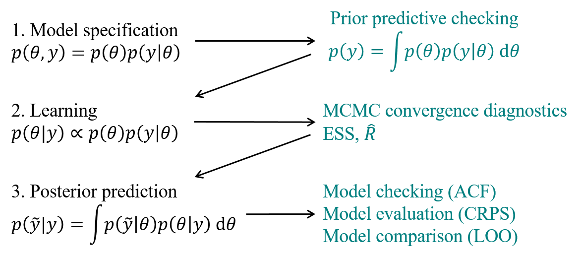
This article starts with a generic tutorial on Bayesian modelling, and shows the essential steps to apply it to building energy use prediction. The following workflow, illustrated on Fig. 15, follows the formalisation into three steps by [Gelman et al., 2013]. Readers interested in a more complete course are referred to this reference book, or the more introductory one of [McElreath, 2018].

Fig. 15 Bayesian data analysis workflow

The methodology is not different from traditional inverse modelling: each candidate model is defined, calibrated, and its validity is checked. All validated models are then ranked on some model comparison metrics, until one is selected. However, Bayesian data analysis comes with probabilistic metrics at each of these steps, which offer greater insight into the reliability of our inferences.

Step 1: setting up a probability model

A full probability model is defined by [Gelman et al., 2013] as a joint probability distribution for observable data \(y\) and unobservable quantities \(\theta\) in a problem.

(2)\[p(\theta,y) = p(\theta)p(y|\theta)\]

where \(\theta\) denote any model parameter, or unobserved quantity, about which to make probability statements. A Bayesian model is therefore defined by two components:

• An observational model \(p(y|\theta)\), or likelihood function, which describes the relationship between the data \(y\) and the model parameters \(\theta\).

• A prior model \(p(\theta)\) which encodes eventual assumptions regarding model parameters, independently of the observed data.

The choice of observational model is up to the expert after data visualisation. Having sensible priors is a way to incorporate scientific knowledge into the model. It can also facilitate convergence of the learning algorithm, should there be identifiability issues from a large number of parameters.

The full probability model is the formalization of many assumptions regarding the data-generating process. In theory, the model can be formulated only based on domain expertise, regardless of the data. In practice, a model which is inconsistent with the data has little chance to yield informative inferences after training. The prior predictive distribution, or marginal distribution of observations \(p(y)\), is a way to check for the consistency of our expertise.

(3)\[p(y) = \int p(y|\theta)p(\theta) \mathrm{d}\theta\]

This is also called the prior predictive distribution. Computing this distribution is equivalent to running a few simulations of a numerical model before its training, by drawing parameter values from a sensible distribution \(p(\theta)\). Prior predictive checks generate data according to the prior in order to asses whether a prior is appropriate [Gabry et al., 2019], if observations are within the realm of possible model outcomes.

At this point of the workflow, no observed data was used in the model definition. In fact, probabilistic modelling could stop here: a model structure has been assumed, parameter probabilities have been chosen, and the prior predictive distribution can be computed for any prediction horizon. This is equivalent to predicting with an untrained model, while propagating the parameter uncertainty expressed by their prior \(p(\theta)\).

Step 2: learning

The target of Bayesian inference is to make probability statements about \(\theta\) given \(y\). Once the full probability model has been specified (Eq. (2)), conditioning on the known value of the data \(y\) using Bayes’ rule yields the posterior density:

(4)\[p(\theta|y) = \frac{p(\theta,y)}{p(y)}\]

(5)\[p(\theta|y) \propto p(\theta) p(y|\theta)\]

It is rarely possible to sample directly from the posterior distribution. Markov Chain Monte Carlo (MCMC) sampling methods are used to stochastically explore the typical set, i.e. the regions of parameter space which have a significant contribution to the desired expectations. Markov chains used in MCMC methods are designed so that their stationary distribution is the posterior distribution. If the chain is long enough, the generated chain \(\left(\theta^{(1)},\dots,\theta^{(S)}\right)\) provides samples from the typical set.

(6)\[\theta^{(s)} \sim p(\theta|y)\]

where each draw \(\theta^{(s)}\) contains a value for each of the \(p\) parameters of the model.

(7)\[\theta^{(s)} = \left(\theta_1,\dots,\theta_p\right)^{(s)}\]

This paper does not aim at explaining MCMC algorithms and their characteristics, but the reader is referred to [Betancourt, 2017] for a description of the state-of-the-art Hamiltonian Monte Carlo (HMC) algorithm and No-U-Turn Sampler (NUTS). Applications of HMC to the calibration of building energy models include whole building simulation [Chong and Menberg, 2018] and state-space models [Lundström and Akander, 2019].

MCMC estimators converge to the true expectation values as the number of draws approaches infinity. In practice, diagnostics must be applied to check that the estimator follows the central limit theorem, which ensures that the estimator is unbiased after a finite number of draws. For that purpose it is first recommended to compute the (split-)\(\hat{R}\) statistic, or Gelman-Rubin statistic, with multiple chains initialized at different initial positions and split into two halves [Gelman et al., 2013]. The \(\hat{R}\) statistic measures for each scalar parameter, \(\theta\), the ratio of samples variance within each chain \(W\) to the sample variance of all combined chains \(B\):

(8)\[\hat{R} = \sqrt{\frac{1}{W} \left(\frac{N-1}{N}W + \frac{1}{N}B \right)}\]

where \(N\) is the number of samples. If the chains have not converged, \(W\) will underestimate the variance, since the individual chains have not had time to range all over the stationary distribution, and \(B\) will overestimate the variance, since the starting positions were chosen to be overdispersed.

Another important convergence diagnostics tool is the effective sample size (ESS), defined as:

(9)\[\text{ESS} = \frac{N}{1 + 2 \sum_{l=1}^{\infty} \rho_l}\]

with \(\rho_l\) the lag-\(l\) autocorrelation of a function \(f\) over the history of the Markov chain. The effective sample size is an estimate of the number of independent samples from the posterior distribution.

The diagnostic tools introduced in this section provide a principled workflow for reliable Bayesian inferences. They are readily available in most Bayesian computation libraries. Based on the recent improvements to the \(\hat{R}\) statistic [Vehtari et al., 2021], it is recommended to use the samples only if \(\hat{R} < 1.01\) and \(\text{ESS} > 400\).

Step 3: model checking and evaluation

The third step of Bayesian data analysis as formulated by [Gelman et al., 2013] is to evaluate the fit of the model and the implications of the resulting posterior distribution. This is done by drawing simulated values from the trained model and comparing them to the observed data.

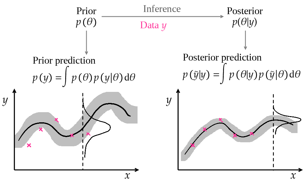
Fig. 16 The posterior predictive distribution are predictions by a model updated with the data

The posterior predictive distribution is the distribution of the observable \(\tilde{y}\) conditioned on the observed data \(y\):

(10)\[p\left(\tilde{y}|y\right) = \int p\left(\tilde{y}|\theta\right) p\left(\theta | y\right) \mathrm{d}\theta\]

This definition is very similar to the prior predictive distribution, except that the prior \(p(\theta)\) has been replaced by the posterior \(p(\theta|y)\). Similarly, it is simple to compute if the posterior has been approximated by an MCMC procedure: a finite number of parameter vectors \(\theta^{(s)}\) is drawn from the posterior distribution, and each of them is used to compute a model output \(\tilde{y}^{(s)}\):

(11)\[\theta^{(s)} \sim p(\theta|y)\]

(12)\[\tilde{y}^{(s)} \sim p(y|\theta^{(s)})\]

where each draw \(\tilde{y}^{(s)}\) contains a value for each of the \(N\) data points of the prediction period.

(13)\[\tilde{y}^{(s)} = \left(\tilde{y}_1,\dots,\tilde{y}_N\right)^{(s)}\]

As a consequence, each individual data point \(i\) has a posterior predictive distribution approximated by the set \(\tilde{y}_i^{(s)}\).

Much like in a traditional model fitting and validation workflow, proper model checking and validation should comprise two steps:

• First, checking the fit of the model with the training data itself through residual analysis. Should the model not match the data on which it was trained, it has little chance for out-of-sample scalability.

• Then, assessing the model’s predictive performance outside of the training data, typically on a dedicated test dataset. The performance metrics used in this second step may then be used to compare and rank several models, and select the “best” one.

Residual analysis

Residual analysis is the process of checking the validity of modelling hypotheses. For instance, if the specification of the observational model states that errors are independent, identically distributed with zero mean and constant variance \(\sigma^2\), then this hypothesis should be checked. One way to do it are the autocorrelation function (ACF) of one-step-ahead prediction residuals, or their cross-correlation function (CCF) with explanatory variables. Residual analysis is often confined to time series models, but is applicable as long as data are time indexed, even if the model does not formulate a dependency between consecutive observations.

The ACF of prediction residuals should have near-zero values for all lags above 1, to indicate the mutual independence of errors. If, for instance, the ACF has a significant non-zero value at lag 24 for a hourly prediction model, there is a chance that a daily occurring phenomenon has not been properly encoded in the model. A visual inspection of the ACF graph is a good diagnosis tool. On a more quantitative note, the Durbin-Watson statistic is used to detect autocorrelation in the residuals at lag 1, and the Ljung–Box test assesses autocorrelation up to a specified number of lags.

Scoring rules

To evaluate a model’s scalability, several metrics may calculated on a test dataset, separated from the training dataset.

The first category of metrics quantify a model’s prediction accuracy. The coefficient of variation of the root-mean-square error (CV(RMSE)) is a well-known measure of point estimates:

(14)\[\mathrm{CV(RMSE)} = \frac{1}{\bar{y}} \sqrt{\frac{1}{N}\sum_{i=1}^N\left(\tilde{y}_i-y_i\right)^2}\]

where \(\tilde{y}_i\) denotes a model prediction, \(y_i\) an observation and \(\bar{y}\) the average of all observations. The (normalized) Mean Bias Error and the Mean Absolute Error are alternatives to the CV(RMSE). However, they all only describe a model’s accuracy, and provide no insight on its precision. With a probabilistic model, these metrics may be calculated using the mean prediction, but more informative metrics are available.

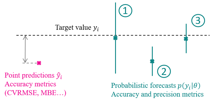
Fig. 17 Assessment probabilistic forecasts. 1) High accuracy, low precision; 2) Low accuracy, higher precision; 3) High accuracy and precision. The second situation is the least favorable: high confidence in an inaccurate solution.

Scoring rules [Gneiting and Raftery, 2007] are model evaluation metrics which assess probabilistic forecasts in terms of both accuracy and precision. They encourage forecasts whose precision match their accuracy: Fig. 17 illustrates the difference between several probabilistic forecasts, compared to a point estimate which can only be assessed by accuracy. The importance of prediction intervals was also underlined by [Chong et al., 2021], who used the Coverage Width-based Criterion metric to assess the reliability of predictions.

The Continuous Ranked Probability Score (CRPS) [Gneiting and Raftery, 2007] is appropriate to use when predictive distributions are expressed in terms of samples, originating from MCMC. Let \(y_i\) be an observation, and \(F_i\) the cumulative distribution function of the posterior prediction for this point \(p\left(\tilde{y}_i|y\right)\). The CRPS between \(y_i\) and \(F_i\) is defined by:

(15)\[\mathrm{CRPS}(F_i, y_i) = -\int_{-\infty}^{\infty} \left( F(z) - \mathcal{H}\left(z\geq y_i\right)\right)^2 \mathrm{d}z\]

(16)\[\mathrm{CRPS}(F_i, y_i) = -\int_{-\infty}^{y_i} F(z)^2 \mathrm{d}z \; - \; \int_{y_i}^{\infty} \left( F(z) - 1\right)^2 \mathrm{d}z\]

where \(\mathcal{H}\) is the Heaviside function which takes a value of 1 if its argument is positive, 0 otherwise. Schematically speaking, the CRPS is the sum of two (squared) areas: between 0 and \(F_i\) for posterior values below \(y_i\), and between \(F_i\) and 1 for values above \(y_i\). A low CRPS is obtained with either a high precision or accuracy, or both (the cumulative distribution varies “quickly” between 0 and 1 near the target value).

The total CRPS of a test dataset is then the sum of individual CRPS values at each data point.

Model comparison and cross-validation

Once a model has passed the validation criteria, its structure may be assumed sufficient to explain the main mechanics of the data generating process. However, this does not ensure that this model is the most appropriate one to draw inferences from, or to use for future predictions.

On one hand, residual analysis imposes a lower bound on the necessary model complexity to capture the data-generating process; on the other hand, an upper bound on model complexity is imposed by the risk of overfitting: a model with too many degrees of freedom will fit the training data very well, but will poorly extrapolate to new data, because it will reproduce specific patterns caused by local errors.

Model selection criteria are designed to help comparing several models, not just based on their fit with training data, but on an estimation of their prediction accuracy with new data. These criteria often reward models that offer a good compromise between simplicity and accuracy. There are several options:

• Computing the above model assessment metrics on a test dataset, separate from the training dataset, gives an estimate of each model’s scalability. However, this ranking still occurs in specific conditions given by the test dataset.

• Cross-validation is similar to this principle: the training data is split into several portions, each of which serves as test data for a model trained on all other portions. \(k\)-fold cross-validation therefore implies fitting a model \(k\) times. Leave-one-out (LOO) cross-validation is the particular case where only one observation is left out of the training dataset.

Exact LOO cross-validation is very costly, since it requires training the model as many times as there are observations, each time leaving out one observation. Instead, Pareto-smoothed importance sampling leave-one-out (PSIS-LOO) cross-validation [Vehtari et al., 2016] approximates the LOO estimate, using the pointwise log-likelihood values computed from samples of the posterior. This method can be considered the state-of-the-art Bayesian criterion of model comparison and selection. It does not require nested models, has a fast computation time and is asymptotically equivalent to the Widely Applicable Information Criterion (WAIC) [Watanabe and Opper, 2010].

The expected log pointwise predictive density for a new dataset (elpd) is a measure of predictive accuracy for the \(N\) data points of a given dataset, taken one at a time. The Bayesian LOO estimate of out-of-sample predictive fit is:

(17)\[\mathrm{elpd}_\mathrm{loo} = \sum_{i=1}^N \mathrm{log}p(y_i|y_{-i})\]

(18)\[p(y_i|y_{-i}) = \int p(y_i|\theta)p(\theta|y_{-i})\mathrm{d}\theta\]

is the leave-one-out predictive density of data point \(y_i\), given the dataset minus the \(i\)th data point, denoted \(y_{-i}\).