Simplified building energy modelling#
Note
This section is incomplete and will be updated progressively along with the tutorials.
The positioning of this book is Bayesian data analysis applied to building energy performance assessment. The first step into this approach, before taking data into consideration, is the probabilistic modelling of the energy balance of buildings. Rather than using Building Energy Simulation (BES) software, our approach is generally to start from simple models and gradually increase complexity if required. This means writing each equation individually, and formulating uncertainty into the probabilistic framework.
Measurement and modelling boundaries#
The first step into setting up a probability model is the choice of its boundaries, i.e. which of the measured data is the dependent variable, and which are the explanatory variables.
The dependent variable \(y\), or model output, is a variable that we wish for a fitted model to be able to predict (this book does not cover situations with several dependent variables in a single model).
The explanatory variables, or independent variables, are the model inputs by which we try to explain the evolutions of the dependent variable. Explanatory variables are denoted \(x\) in most regression models, or \(u\) in more complex hierarchical models where \(x\) may denote a latent variable instead.
The IPMVP defines measurement boundaries as “notional boundaries drawn around equipment, systems or facilities to segregate those which are relevant to saving determination from those which are not. All Energy Consumption and Demand of equipment or systems within the boundary must be measured or estimated. […] Any energy effects occurring beyond the selected measurement boundary are called interactive effects. The magnitude of any interactive effects needs to be estimated or evaluated to determine savings associated with the ECMs.”

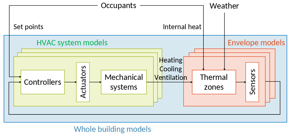
Fig. 13 A slightly more elaborate formalisation of a building.#
The same definition of boundaries work for simulations: a model must be defined so that its inputs and outputs are the measured independent and dependent variables, and all energy effects occurring within these boundaries are either fixed, or part of the list of parameters \(\theta\) that will be estimated by calibration.
Fig. 13 proposes a decomposition of a building into three main categories of models, with different scopes and purposes, that we will cover in tutorials.
Some models are focused on a single thermal zone. They solve its energy balance by receiving its heating, cooling and ventilation loads as input, and compute the indoor temperature. The target of these models is often the characterisation of the envelope’s heat transfer coefficient. RC models, covered later in this book, belong in this category. HVAC systems are usually not in the modelling boundary.
Whole building models take weather files and occupancy information (set points, schedules, internal heat gain) as input. These models range from very simplified (energy signature models) to detailed BES. The dependent variable can be energy consumption recorded by meters, or heating and cooling loads if such measurements are available.
For the purpose of fault detection and diagnosis, models focused on a single system are possible, if measurements are available on its boundaries.
Building physics in a nutshell#
BES decomposes a building into separate thermal zones, each of which is assumed to have a uniform air temperature. A single-family house may be split into one or two zones, while larger housings and office buildings have more, usually denoted by their orientation and usage. The temporal evolution of temperature, humidity and other variables of comfort or indoor air quality, are calculated in each zone as consequences of: influence of the weather; exchange between zones; HVAC settings; occupancy. BES software can reach quite a high level of detail when modelling the phenomena that influence these indoor variables: long-wave radiative heat exchange between all walls; position of the sunspot; influence of furniture on indoor humidity; CFD modelling of air flow…
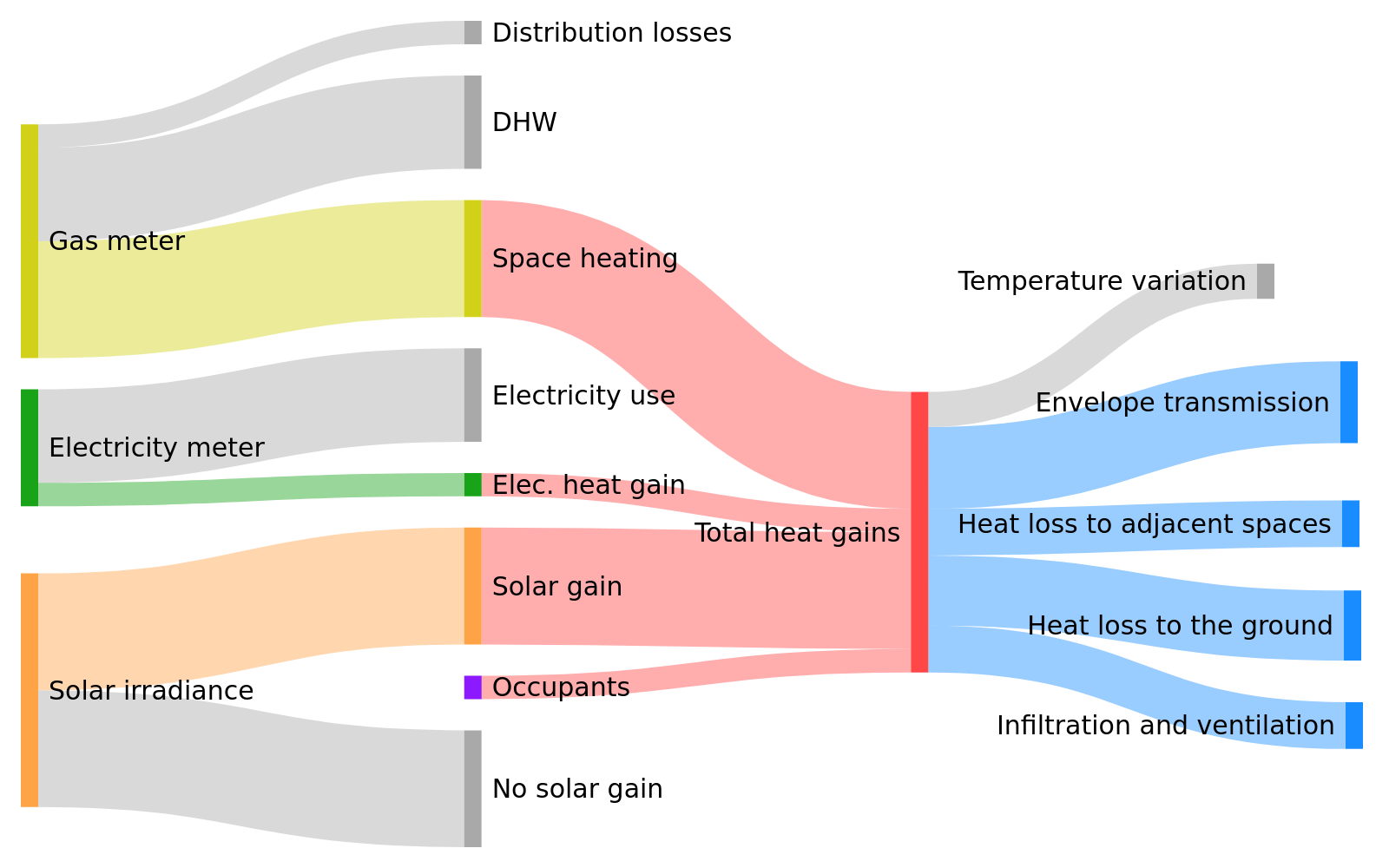
Since we will give our building energy models a probabilistic formulation, these models should stay as simple as possible, while staying close to the main phenomena that govern the heat and energy balance of an observed building. A schematic outlook of heat gains and losses in a heated space is shown on Fig. 14 on the example of a heated building in which gas is the main fuel used by the heating appliances. A similar reasoning can be done in other conditions, such as an air conditioned building in summer.

Fig. 14 Decomposition of heat gain and loss in a heated zone#
